Controllability of LTI System

Consider the following system: \[ \begin{align} \dot{x}(t) &= Ax(t) + Bu(t) \\
y(t) &= Cx(t) \end{align} \] where \(x(t)\in \mathbb{R}^{N+M}, u(t) \in \mathbb{R}^{S}, y(t) \in \mathbb{R}^{M}\). Consequently, \(A\in\mathbb{R}^{(N+M)\times(N+M)}, B\in \mathbb{R}^{(N+M)\times S}, C\in \mathbb{R}^{M\times(N+M)}\).

The controllability of this system can be given by Kalman’s Criterion: \[rank(K) = rank([CB,CAB,CA^{2}B,\ldots,CA^{N+M-1}B]) = M\] In another words, controllability matrix \(K\) needs to have full row-rank. This criterion is highly intuitive and follows from a simple derivation:

Consider the above system, by looking into higher order derivative of the system we get that (omitting \((t)\)): \[ \begin{align} & \dot{x} = Ax + Bu \\\
& \ddot{x} =\frac{d}{dt}(Ax+Bu) = A\dot{x} + B\dot{u} = A^{2}x + ABu + B\dot{u} \\\
& \cdots \\\
& x^{(N+M-1)} = A^{N+M-1}x + A^{N+M-2}Bu + A^{N+M-3}Bu^{(1)} + \ldots + Bu^{(N+M-2)} \\\
\end{align} \]

Therefore, we have \[ x^{(N+M-1)}-A^{N+M-1}x = \begin{bmatrix} A^{N+M-2}B & A^{N+M-3}B & \ldots & B \end{bmatrix} \begin{bmatrix} u \\\ u^{(1)} \\\ \vdots \\\ u^{(N+M-2)} \end{bmatrix} \] Similarly by rearranging the terms in the matrices in reverse orders, \[ y^{(N+M-1)}-CA^{N+M-1}y = \begin{bmatrix} CB & CAB & \ldots & CA^{N+M-2}B \end{bmatrix} \begin{bmatrix} u^{(N+M-2)} \\\ u^{(N+M-3)} \\\ \vdots \\\ u \end{bmatrix} \]

Let \begin{equation} \mathbf{z} = y^{(N+M-1)}-CA^{N+M-1}y \\
K = \begin{bmatrix} CB & CAB & \ldots & CA^{N+M-2}B\end{bmatrix} \\
\mathbf{u} = \begin{bmatrix}u^{(N+M-2)} \\\ u^{(N+M-3)} \\\ \vdots \\\ u \end{bmatrix} \end{equation} , we have \[\mathbf{z} =K\mathbf{u} \]

Naturally, for solution \(\mathbf{u}^{\star}\) to exist for any given \(\mathbf{z}\), we require matrix \(K\) to have full row-rank. In fact, because the matrix \(K\) is generally “fat” - have more rows than columns, there will exist inifinite number of solutions since the null-space of the system is non-trivial. This could be desirable for the case of control because it means that there are infinite number of solutions of the form \(\mathbf{u} = \mathbf{u}^{0} + \mathbf{\tilde{u}}, \mathbf{\tilde{u}}\in null(K)\) which can satisfy our linear system.

However, in most systems where the exact values of the matrices \(A,B,C\) are only known to the extent of if they are zero, the above Kalman criterion cannot be evaluated, we require the notion of structural controllability, which was introduced by Ching-Tai Lin in 1974.

Structural Controllability

Structural Controllability deals with strucutral matrices where the entries of the matices are either: fixed zeros or free non-zero parameters. Such notion of controllability is extremely useful for network control analysis with sparse connectivity, meaning the \(A,B,C\) matrices have mostly zero entries. Note also that, if system is structurally controllable, it is controllable with almost all possibly values of nonzero entries of \(A,B,C\) except for pathological cases, in which case small perturbations of the parameters will get rid of the uncontrollability.

To evaluate structural controllability of a system, it is often useful to consider the network where vertices are the \(n\) nodes and edges are the non-zero entries of the system matrices.

Following the setup of the original paper by Lin, we consider an alternative system of the form characterized by two matrices \((A,b)\): \[\dot{x} = Ax + bu, x \in \mathbb{R}^{n}, u \in \mathbb{R} \]

The paper states the following important results:

the pair \((A,b)\) is structurally controllable if and only if the graph of \((A,b)\) is “spanned by a cactus”

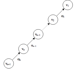
A cactus is a network created using “stems” and “buds”, which are fundamental network structures that are both structurally controllable. A stem corresponds to the following system \[ A = \begin{bmatrix} 0 & \alpha_{1} & 0 & \dots & 0 \\
0 & 0 & \alpha_{2} & \dots & 0 \\
\vdots & \vdots & \vdots & \ddots & \vdots \\
0 & 0 & 0 & \dots & \alpha_{n-1}\\
0 & 0 & 0 & \dots & 0 \end{bmatrix} , b = \begin{bmatrix} 0 \\
0 \\
\vdots \\
0 \\
\alpha_{n} \end{bmatrix} \]

Plotting the graph of the augmented system \((A,b)\), we get the following:

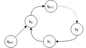
Similarly we have a bud corresponding to the following system \[ A = \begin{bmatrix} 0 & \alpha_{1} & 0 & \dots & 0 \\
0 & 0 & \alpha_{2} & \dots & 0 \\
\vdots & \vdots & \vdots & \ddots & \vdots \\
0 & 0 & 0 & \dots & \alpha_{n-1}\\
\alpha_{n+1} & 0 & 0 & \dots & 0 \end{bmatrix} , b = \begin{bmatrix} 0 \\
0 \\
\vdots \\
0 \\
\alpha_{n} \end{bmatrix} \]

Plotting the graph of the augmented system \((A,b)\), we get the following:

The process of creating a cactus from stems and buds is governed by the following lemma (Lemma 1 of Lin 1974):

Suppose that \(G\) is a graph of structurally contorllable pair (system). Let \(B\) be a bud with the origin \(e\), and suppose \(e\) is the only node which belongs at the same time to the vertex set of \(G\) and to the vertex set of \(B\), then \(G\cup B\) is the graph of a structurally controllable pair.

Alternatively, suppose bud \(B = B(e)\) where \(e\) is its origin, then \(G\cup B\) is the graph of a structurally controllable pair if \(B(e) \cap G = e\).

Central Question

The central question of network control using structural controllability is

Given topology of control network: (1) how many output nodes are controllable, (2) which intermediate nodes are essential/non-essential.

Linking Graph

To incorporate the notion of time to this control system, the system is unrolled in time to form a linking graph with discretized time steps. Specifically, we create \(G_{linking} = G_{linking}(A,B,C)\) defined on the three structural matrices. The vertex set of \(G_{linking} = V_{A}\cup V_{B} \cup V_{C}\), where \(\begin{align} V_{A} & = \{v^{A}_{i,t} | i = 1,2,\ldots,N+M; t = 1,2,\ldots,N+M\} \\ V_{B} & = \{v^{B}_{i,t} | i = 1,2,\ldots,S; t = 1,2,\ldots,N+M-1\} \\ V_{C} & = \{v^{C}_{i} | i = 1,2,\ldots,M\} \end{align}\)

And the edge set \(E = E_{A} \cup E_{B} \cup E_{C}\) is given by: \(\begin{align} E_{A} & = \{v^{A}_{j,t}\rightarrow v^{A}_{i,t+1} |a_{ij}\neq 0, t = 1,2,\ldots,N+M-1\} \\ E_{B} & = \{v^{B}_{j,t}\rightarrow v^{A}_{i,t+1} |b_{ij}\neq 0, t = 1,2,\ldots,N+M-1\} \\ E_{C} & = \{v^{A}_{j,t}\rightarrow v^{C}_{i} |c_{ij}\neq 0, t = N+M\} \end{align}\)

The linking size of \(G_{linking}\) is the maximum number of disjoint paths from node set \(V_{B}\) to \(V_{C}\). Here, disjoint means that these path do not have any common vertices. It has been established that the structurally controllable number of nodes of the original system \((A,B,C)\), say \(z\) is upper bounded by the linking size of the dynamic graph \(G_{linking}\):

\[z\leq z^{\star}\]